Pipe pile caps have been around as long as pipe piles, but mating them to a pile hammer via a pipe cap may be new to some users. The diagram above (which, as you can see, dates from 1931) shows how this is done. The cross-section shows three diameters of pipe piles mating with a … Continue reading Mating Pipe Piles to Pipe Pile Caps
Pulling Adapters for Vulcan Extractors
Vulcan pile extractors were largely designed to extract sheet piling. The standard connection had two (2) or three (3) holes that needed to be burned into the sheeting. While this provided a very durable connection, it was time consuming and is not really applicable to piling such as wood piling. Above is a diagram, taken … Continue reading Pulling Adapters for Vulcan Extractors
New Version of TAMWAVE Online Wave Equation Program Now Available
TAMWAVE 7: Analysis for a Cohesive Soil
With the analysis of the concrete pile in cohesionless soils complete, we turn to an example in cohesive soils.
The analysis procedure is exactly the same. We will first discuss the differences between the two, then consider an example.
Differences with Piles in Cohesive Soils
- The unit weight is in put as a saturated unit weight, and the specific gravity of the soil particles is different (but not by much.)
- Once the simulated CPT data was abandoned, the “traditional” Tomlinson formula for the unit toe resistance, namely $latex q_t = N_c c $, where $latex N_c = 9 $, was chosen.
- The ultimate resistance along the shaft is done using the formula of Kolk and van der Velde (1996). This was used as a beta method, for compatibility with the method used for cohesionless soils. Unless the ratio of the cohesion to the effective stress is constant, the…
View original post 3,746 more words
TAMWAVE 6: Results of Wave Equation Analysis
With the data entered for the wave equation analysis, we can now see the results. There’s a lot of tabular data here but you need to read the notes between it to understand what the program is putting out. If you are not familiar at all with the wave equation for piles, you need to review this as well.
| Time Step, msec | 0.04024 |
| Pile Weight, lbs. | 15,000 |
| Pile Stiffness, lb/ft | 600,000 |
| Pile Impedance, lb-sec/ft | 57,937.5 |
| L/c, msec | 8.04688 |
| Pile Toe Element Number | 102 |
| Length of Pile Segments, ft. | 1 |
| Hammer Manufacturer and Size | VULCAN O16 |
| Hammer Rated Striking Energy, ft-lbs | 48750 |
| Hammer Efficiency, percent | 67 |
| Length of Hammer Cushion Stack, in. | 16.5 |
| Soil Resistance to Driving (SRD) for detailed results only, kips | 572.7 |
| Percent at Toe | 35.39 |
| Toe Quake, in. | 0.220 |
| Toe Damping, sec/ft | 0.07 |
For those familiar with the…
View original post 2,482 more words
TAMWAVE 5: Wave Equation Analysis, Overview and Initial Entry
With the static analysis complete, we turn to the wave equation analysis. TAMWAVE (as with the previous version) was based indirectly on the TTI wave equation program. Although the numerical method was not changed, many other aspects of the program were, and so we need to consider these.
Shaft and Toe Resistance
Most wave equation programs in commercial use still use the Smith model for shaft and toe resistance during impact. Referencing specifically their use in inverse methods, Randolph (2003) makes the following comment:
Dynamic pile tests are arguably the most cost-effective of all pile-testing methods, although they rely on relatively sophisticated numerical modelling for back-analysis. Theoretical advances in modelling the dynamic pile-soil interaction have been available since the mid-1980s, but have been slow to be implemented by commercial codes, most of which still use the empirical parameters of the Smith (1960) model. In order to allow an appropriate…
View original post 1,087 more words
TAMWAVE 4: Shaft Resistance Profile, ALP and CLM2
With the basic parameters established, we can turn to the static analysis of the pile, both axial and lateral.
Shaft Resistance Profile
| Depth at Centre of Layer, feet | Soil Shear Modulus, ksf | Beta | Quake,inches | Maximum Load Transfer, ksf | Spring Constant for Wall Shear, ksf/in | Smith-Type Damping Constant, sec/ft | Maximum Load Transfer During Driving (SRD), ksf |
| 0.50 | 48.4 | 0.163 | 0.0022 | 0.009 | 4.03 | 45.394 | 0.009 |
| 1.50 | 83.9 | 0.163 | 0.0038 | 0.027 | 6.99 | 19.911 | 0.027 |
| 2.50 | 108.3 | 0.163 | 0.0050 | 0.045 | 9.02 | 13.572 | 0.045 |
| 3.50 | 128.1 | 0.163 | 0.0059 | 0.063 | 10.68 | 10.543 | 0.063 |
| 4.50 | 145.3 | 0.163 | 0.0067 | 0.081 | 12.11 | 8.730 | 0.081 |
| 5.50 | 160.6 | 0.164 | 0.0074 | 0.098 | 13.38 | 7.509 | 0.098 |
| 6.50 | 174.6 | 0.164 | 0.0080 | 0.116 | 14.55 | 6.623 | 0.116 |
| 7.50 | 187.6 | 0.164 | 0.0086 | 0.134 | 15.63 | 5.948 | 0.134 |
| 8.50 | 199.7 | 0.164 | 0.0091 | 0.152 | 16.64 | 5.414 | 0.152 |
| 9.50 | 211.1 | 0.164 | 0.0097 | 0.170 | 17.59 | 4.980 | 0.170 |
| 10.50 | 222.0 | 0.164 | 0.0102 | 0.188 | 18.50 | 4.618 | 0.188 |
| 11.50 | 232.3 | 0.164 |
View original post 1,756 more words
TAMWAVE 3: Basic Results of Pile Capacity Analysis
With the soil properties and lateral loads finalised, we can proceed to look at the program’s static results. These are shown below. We will concentrate on cohesionless soils in this post; a sample case with cohesive results will come later.
| Pile Data | |
| Pile Designation | 12 In. Square |
| Pile Material | Concrete |
| Penetration of Pile into the Soil, ft. | 100 |
| Basic “diameter” or size of the pile, ft. | 1 |
| Cross-sectional Area of the Pile, ft2 | 1.000 |
| Pile Toe Area, ft2 | 1.000 |
| Perimeter of the Pile, ft. | 4.000 |
| Soil Data | |
| Type of Soil | SW |
| Specific Gravity of Solids | 2.65 |
| Void Ratio | 0.51 |
| Dry Unit Weight, pcf | 109.5 |
| Saturated Unit Weight, pcf | 130.5 |
| Soil Internal Friction Angle phi, degrees | 32 |
| Cohesion c, psf | |
| SPT N60, blows/foot | 20 |
| CPT qc, psf | 211,600 |
| Distance of Water Table from Soil Surface, ft. | 50 |
| Penetration of Pile into Water Table, ft. | 50 |
View original post 1,894 more words
TAMWAVE 2: Modifying the Soil Properties
With the first step out of the way, we can proceed to the second: allowing the user to modify the properties of the soil. This option must be used with care since it is easily possible to put together a set of soil properties that is physically unrealistic if not impossible.
Also, if you have chosen a sand or clay, you have chosen the methodology you will use. Adding cohesion to a sand or gravel, for example, will have no effect on the subsequent performance of the model.
Finally, depending upon the choice of a free or fixed head, you are given the option of entering lateral loads and/or moments for the pile head. In this case we have opted to add a lateral load of 10 kips to the pile and no moment. The default is zero for both load and moment; this will produce some coefficients but…
View original post 5 more words
TAMWAVE 1: Entering Basic Soil and Pile Properties
With a few preliminaries out of the way, we can proceed to discuss the new TAMWAVE routine, which can be found here.
What is TAMWAVE?
TAMWAVE stands for Texas A&M Wave Equation. The TTI wave equation was developed at Texas A&M in the late 1960’s and early 1970’s, and was a successor to Smith’s original wave equation program. In reality this is more than a wave equation program; it is a driven pile analyser which, in addition to the wave equation program, analyses the static performance of a driven pile for both axial and lateral loads. It is not intended to be used on actual projects, but as an educational tool for students. Most of the software in current use is expensive, and predecessors such as SPILE, WEAP87 or COM624 are hard to use (they’re DOS programs) or methodological obsolescence issues. (With WEAP87, there are not as…
View original post 832 more words

