As we saw in the previous post, Sanders’ Formula wasn’t the last word in dynamic formulae, and neither were Weisbach’s. Faced with this proliferation, the U.S. Army Corps of Engineers put together the document Pile Foundations and Pile-Driving Formulae, Circular No. 17, Office of the Chief of Engineers, U.S. Army. It was dated 28 November 1881, a month before the Warrington brothers finalised the incorporation of the Vulcan Iron Works and returned the company to the family’s hands. It is not a formal technical paper but a record of reminiscences from several hands combined with analysis of jobsite data from a project thirty years in the past. It showed that the driven pile community was beginning to grasp some of the complexities of the oldest type of deep foundations, both during installation and in use. It also showed that the community had a long way to go in grasping these complexities, a journey that has not ended yet.

The Project

Coastal defences were a major preoccupation of U.S. Army Engineers during the nineteenth century. Defending a long coastline (which became longer with territorial expansions such as Florida, the Louisiana Purchase, the incorporation of the Republic of Texas and the securing of the West Coast from Britain and Mexico) was a large part of the mission of the American military, both Army and Navy. Since by definition coastal forts are near the water, virtually all of them were supported on driven piles. The first two dynamic formulae used in the U.S. were used at Fort Delaware (on the river with that name) and Fort Montgomery (on Lake Champlain.)

The location of the jobsite was at Proctorsville, LA, shown in Figure 1, which dates from 1879. The monograph refers to this as the “Martello Tower,” and it’s called out on the chart as the “Martello Castle.” This is a close in time to the job (1856-7) as I could find; because of changes in South Louisiana geography from then until now, it is best to use a chart as contemporaneous to the project as possible. It is evident that the objective of putting a fort in this otherwise remote location was to prevent sea attack via Lake Borgne (which is indirectly connected to the Gulf) as opposed to up the Mississippi River, as the British had done in the War of 1812 and the Union would do during the Civil War. That great conflict divided the time of the project to the time of the report; in some ways, the Civil War was to dynamic formulae what World War II would be to the wave equation.

Most of the account of the project was set down by Major G. Weitzel, but the overall commander of the job was Brevet Major P.G.T. Beauregard, who was also in charge of building the New Orleans Custom House. (Yes, it is the same Beauregard who served in the Confederate Army, and whose first action was to fire on Fort Sumter in Charleston, SC, yet another coastal fortification.)

The Dynamic Formulae

Before we plough into the specifics of the piling, first there are three terms which appear in the Corps’ report and other monographs of the time that need some definition:

• “Power” does not refer to work in a period of time (as we define it now) but is generally a force applied to a body or system. This definition appears in elementary textbooks of the period such as Smith’s Mechanic, with worked examples.
• “Fall” is the distance a drop hammer descends to impact the pile. We generally refer to this distance as a “stroke” but this is more accurately applied to “automatic hammers” (hammers which raise and in some cases lower their own rams) and not drop hammers.
• “Ton” in this time was generally what we call the “long ton” or “Imperial ton” of 2,240 pounds.

A concept that was well established was ASD (Allowable Stress Design) and the distinction between the ultimate and allowable pipe axial capacities, related by a factor of safety. Although the terminology used at the time differs from ours—and the factor of safety is frequently inverted—the idea is basically the same.

The formulae featured in the study were a mixed bag in terms of their construction. All were empirical to varying degrees. Some (McAlpine, Trautwine) were purely empirical with no attempt for consistent units. Unit analysis could be applied to the rest.

Sanders’ Formula

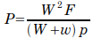
Sanders’ Formula for the ultimate capacity of the pile is simply

where P is the ultimate load of the pile, F is the fall of the ram, W is the weight of the hammer, and p is the set for the last blow of the hammer. P and W are in the same units of force and F and p are in the same units of length. Generally, Sanders’ Formula was used with a factor of safety. For a factor of safety of 8, for example, it becomes

and P becomes the allowable load of the pile.

Weisbach/Mason Formula

For all of the mathematical prowess Weisbach showed in this post, the formula attributed to Weisbach by Weitzel was generally of the form

where P, W, F and p are the same as Sanders’ Formula and w is the weight of the pile. A little algebra will reduce this formula to

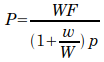
It is basically Sanders’ Formula with provision for the ratio of the pile weight to the ram weight. It was the formula used by Mason in the construction of Fort Montgomery.

McAlpine’s Formula

McAlpine (who used this in the construction of the Brooklyn Dry Dock) computed the ultimate capacity as follows:

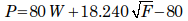
where P is the ultimate capacity of the pile in tons, W is the weight of the ram in tons and F is the fall in feet. It is the only formula I am aware of which does not consider the pile set per blow or blows per inch or foot of penetration. It can also yield a negative result if the values of W and F together are not sufficiently large (the Gates formula is also capable of negative results.)

Trautwine’s Formula

The Trautwines were one of the most prominent families in American civil engineering; the formula below was set forth by the junior John C. Trautwine:

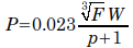
where P is the ultimate capacity of the pile in tons, F is the fall of the ram in feet, W is the weight of the ram in pounds, and p is the set of the last blow of the pile in inches. The formula differed from both Sanders and the Weisbach “family” of formulae in the following ways:

• The cube root of the drop height was used. Sanders had assumed that the penetration of the pile was directly proportional to the energy output of the hammer. Trautwine’s formula penalised hammers with long strokes and light ram weights (such as drop hammers,) an issue which is very much with us today.
• Trautwine added an additive constant to the denominator, which prevented the ultimate load from going to infinity with zero set. This solved a practical weakness of the previous formulae.

In the years after the Civil War, the Trautwine formula was probably the most used alternative to the Sanders and Weisbach family formulae.

Nystrom’s Formula

Weitzel has evidently messed up Nystrom’s Formula; if we use the form according to Goodrich (1908),

or

It is basically Weisbach’s Formula with a different provision for the pile to ram weight ratio. The variables are the same.

Rankine’s Formula

Dynamic formulae, desultory of a business that they were, occupied the great minds of civil engineering, and in this era no greater a one than Rankine. His formula was as follows:

In consistent units, variables are the same as Sanders’ Formula except for e (modulus of elasticity of pile) and s (cross-sectional area of pile.)

The formulae presented here are as they apply to this study. There was considerable cross-fertilisation (and confusion) with the various formulae and their attributions, a situation further complicated by the way factors of safety were applied, as we will see.

Overview of the Project

The best overview of the project is that of Weitzel himself:

The site of the tower at Proctorsville, as determined by actual borings, was found to have the following character, viz.: For a depth of nine feet there was mud mixed with sand, then followed a layer of sand about five feet thick, then a layer of sand mixed with clay from four to six feet thick, and then followed fine clay. Sometimes clay was met in small quantities at the depth of six feet, as well as small layers of shells. By draining the site the surface was lowered about six inches.

The foundation piles were driven in a square of twenty piles on a side, four feet from centre to centre. Twenty-four were omitted to leave room for fresh water cisterns, and two extra ones were driven to strengthen supposed weak ones. The total number at first driven was therefore 378. The piles were driven to distances varying from 30 to 35 feet below the surface, or from 10 to 15 feet into the clay stratum. The average number of blows to a pile was 55, and mainly hard driving. After all these piles were driven, ten additional ones were driven at different points to strengthen supposed weak points. Each one of them required over 100 blows to drive it.

The boring strikes us today as vague and unscientific, but the fact that it done at all was a plus.

Test Pile Program: Results and Analysis of Dynamic Formulae

Before production piles were started a test pile was driven and analysed. The test pile was as follows:

Before beginning the foundation I drove an experimental pile exactly in the centre of the site. It was 30 feet long, 12 ½” x 12″ at top and 11 ½” x 11” at butt. It was sharpened to a bottom surface about 4 inches square. Its head was capped with a round iron ring. Its weight was 1,611 pounds and the weight of the hammer was 910 pounds. Its own weight sank it 5′ 4″, and it required 64 blows to drive it 29′ 6″ deeper. The fall of the hammer at the first blow was 6 feet, increasing each successive blow by the amount of penetration, excepting the last ten blows when the fall was regulated to exactly 5 feet at each blow.

The simplest way to illustrate the blow count history—which is given in the narrative—is to do so the way we would do it now, with a graph as shown in Figure 2.

In looking at this, it needs to be kept in mind that, with a drop hammer, if the pile starts towards the top of the rig, the rig is not moved and the top of the stroke is held constant, the stroke will increase as the pile is driven into the ground. As the stroke was not regulated until the last ten blows, what looks to be the pile “taking up” is more likely a decrease in set with a decrease in the stroke. Lack of “take-up” or reaching a competent layer is not unusual in a South Louisiana stratigraphy.

The test pile driven, it was then load tested as follows:

This pile, according to Colonel Mason’s formula, should have borne 52,556 pounds. I loaded it with 59,618 pounds and it did not settle. I afterwards increased the load to 62,500 pounds, when it settled slowly. The greatest weight to be carried by any one pile was between 30,000 and 35,000 pounds.

This illustrates one of the major problems at the time in verifying the dynamic formulae: static load testing did not have a standard method either of performance or of interpretation. The object of a static load test at the time was to determine whether the piles would withstand a certain test load (obviously based on the service load) with an acceptable settlement, that acceptability varying from structure to structure. Although we have standardised both the testing and interpretation methods, our methodology of either is not truly univocal.

Dynamic Formula Verification and Factors of Safety

One of the purposes of the 1881 document was to examine the results of the Proctorsville test in light of a number of dynamic formulae. A table was assembled with the results of these formulae for the final blow count. In order to put these results in a broader perspective, a bearing graph type of comparison was assembled and is shown in Figure 3.

All of the formulae (including Sanders) were evaluated at their ultimate values, without application of a factor of safety. The only variable parameter is the blow count/pile set; the other parameters are shown in Table 1.

Ram Weight	910	pounds
Ram Weight	0.41	tons
Fall of Hammer	5	feet
Fall of Hammer	60	inches
Pile Weight	1611	pounds
Pile Weight	0.72	tons
Modulus of Elasticity	750	tsi
Modulus of Elasticity	1680000	psi
Area of Pile Head	150	sq.in.
Area of Pile Toe	126.5	sq.in.
Average Cross-Sectional Area	138.25	sq.in.
Pile Length	30	feet
Pile Length	360	inches

Some comments on Figure 3 are as follows:

• The Sanders, Mason/Weisbach and Nystrom formulae show a linear increase in ultimate capacity with blow count. This is obviously defective; both experience and analysis shown a diminishing returns phenomenon as a pile is driven. The concept that beating on a pile at refusal can achieve any required increase in capacity has broken many piles and contractors.
• The other two formulae show the flattening of the curve with increasing blow count, the Trautwine formula more so than the Rankine one.
• All of these results are ultimate; to obtain an allowable capacity, it is necessary to apply a factor of safety. But which factor of safety? That depends upon the static load whose settlement is acceptable, and also the required design load of the pile itself. Based on the static load test data (such as it is,) the required design load of 30-35 kips is more than achieved with an acceptable static load of around 60 kips, which implies a factor of safety of around 2. The result is probably due to the design being made based on experience and then verified using a static load test program without reliance on the dynamic formulae. Adding the dynamic formulae to the mix shows that, in this case, the Trautwine and Mason/Weisbach formulae are closest to the static load test results. Given the scatter of the formulae current at the time, such a match is best seen as being made in hindsight.

The factor of safety question becomes more complicated in the notional pile study which Elliot conducted. The number of “different” formulae was increased to twenty and both ultimate and allowable capacities were computed. A cursory examination of this part of the report will show that factors of safety vary wildly from formula to formula and even with the same formula promulgated by a different person. At the end of his report Elliot recommends the following:

From the foregoing considerations, I come to the following conclusions:

1st. Pile driving formulae should be accompanied by tables of factors of safety, corresponding to all the common and easily recognizable kinds of soil.

2nd. These factors of safety should be determined on after extended experiments on the supporting power of piles, although approximate factors which could be used without hazard, could be found from examinations of the records of the driving of the piles of actual foundations, provided the weights of the superstructures are known, and descriptions of the soils have been preserved; and provided also, that the foundations have carried their loads during sufficient lengths of time.

Unfortunately adding to the complexity of determining the factor of safety, combined with the variable basis of the dynamic formulae current at the time (and those subsequently developed) also added to the confusion. This aspect is frequently overlooked in discussions of the weaknesses of dynamic formulae. Using a static load test to calibrate a dynamic formula on a job to job basis did become a common practice, one which has influenced pile design to the present time.

Pile-Soil Interaction

In the course of considering the dynamic formulae, some consideration to pile-soil interaction was given, especially for how much the soil was a part of the moving pile during impact. But this in turn brought up the subject of load transfer from the pile to the soil, which occasioned this line of thinking:

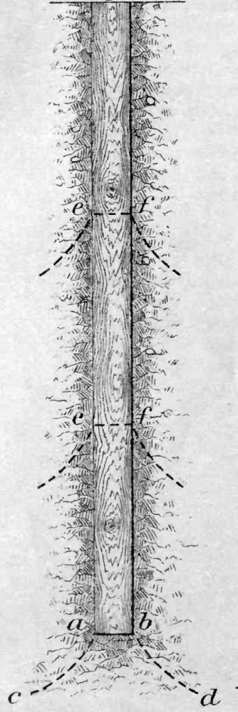
Let us see what supports a loaded pile.

I conceive that there is below the bottom of the pile in ordinary soils, a conoidal mass of earth, a, b, c, d, (Figure 4) the particles of which are acted upon by pressures derived from the weight of the pile and its load, and the form and dimensions of which, depend on this weight and on the kind of soil; that at every section e, f; e, f, of the pile below the surface of the ground, the particles of earth in contact with the pile, are, by reason of friction, pressed downward, and that these pressures are distributed (spread) in the same way that the pressure at the foot of the pile is distributed ; that is, through the particles of the earth surrounding the pile, which are limited by conoidal surfaces, of which, (in homogeneous soils,) the pile is a common axis.

Much of what follows isn’t very specific, but this problem has occupied geotechnical engineers for many years. With the toe the bearing capacity model has been applied but not without detractors; however, it should be remembered that shallow foundation bearing capacity theory was still in the future at the writing of this report. As for the interaction between the pile and soil during impact is concerned, the following statement was prescient:

When these comparisons in the case of any kind of soil have been made, the true relation between these effects and these results may be discovered, and correct and reliable factors of safety for use with formulae for the sustaining power of piles, into which formulae enter the terms common to all pile driving formulae, (viz., the weight of the ram, its fall, and the average penetration of the last blows,) may be made for that kind of soil, but I think it evident that no pile driving formula or factors of safety based only on theoretical deductions from the formula Ps = Mv²/2 , can be relied on, even for single isolated piles, or for piles driven at considerable distances apart.

Pile Set-Up After Driving

Another issue that came into focus during the analysis was the change in pile capacity from the time of driving to the time the actual service load was applied. One Col. Comstock weighed in on this as follows:

The formulae only consider the resistance during the very short period of the blow. It would be strange if such resistance were always, for all soils, the same as when, sometime after the pile had been driven, it was loaded until it began to move. Possibly the latter resistance is sometimes the greater, usually it is doubtless much less, for most materials require a less force to change their form slowly than rapidly. A substance like clay, that is plastic, might resist driving piles very strongly and yet furnish a very much smaller resistance to a permanent load.

Not knowing the relation of the two resistances, a formula which does not include that relation (i.e., the character of the soil), may be, even for isolated piles, much in error. The only way to get a reliable formula seems to be to determine for characteristic, well defined, and carefully described soils, the ratio between the resistances given by some good formula like Rankine’s, and the actual load which will start the pile very slowly down and keep it going.

Comstock conflated two different problems into one: the effect of the high loading rate during impact on the soil resistance to driving (SRD,) and the effects of soil changes on pile capacity after driving. Smith’s wave equation incorporated a velocity-dependent component to the SRD, the determination of which is a very important component in a successful wave equation analysis. The second problem—pile set-up, mostly due to elevated pore water pressures from driving being slow to dissipate due to low permeability soils—is one that continues to occupy driven pile research. The two problems are different and need separate treatments, which they receive today.

Pile Group Capacity

Since the piles at Proctorsville were driven as a group, the relationship between single and group pile capacity became a topic of importance. Because of the lower capacity of wood piles, large groups of piles were frequent. About this Elliot noted the following:

Now let us examine the case of an ordinary pile foundation in any compressible soil. Say that the piles are driven three (3) feet apart, in rows the same distance apart, from centre to centre.

Would a safe load for this foundation be equal to the safe load of a single isolated pile in that soil, multiplied by the number of piles?

I think not, for, if it be true that below and surrounding the piles, there exist within the soil the conoids of pressure before alluded to, and if the surfaces of these conoids make any considerable angle with the vertical, then the pressure upon the earth below and between the piles, may be much greater in the case supposed, than in the case of an isolated pile.

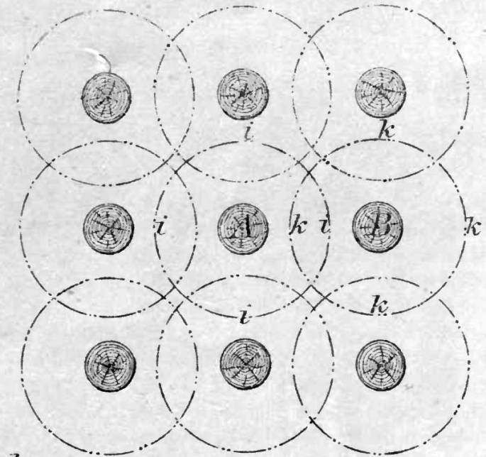
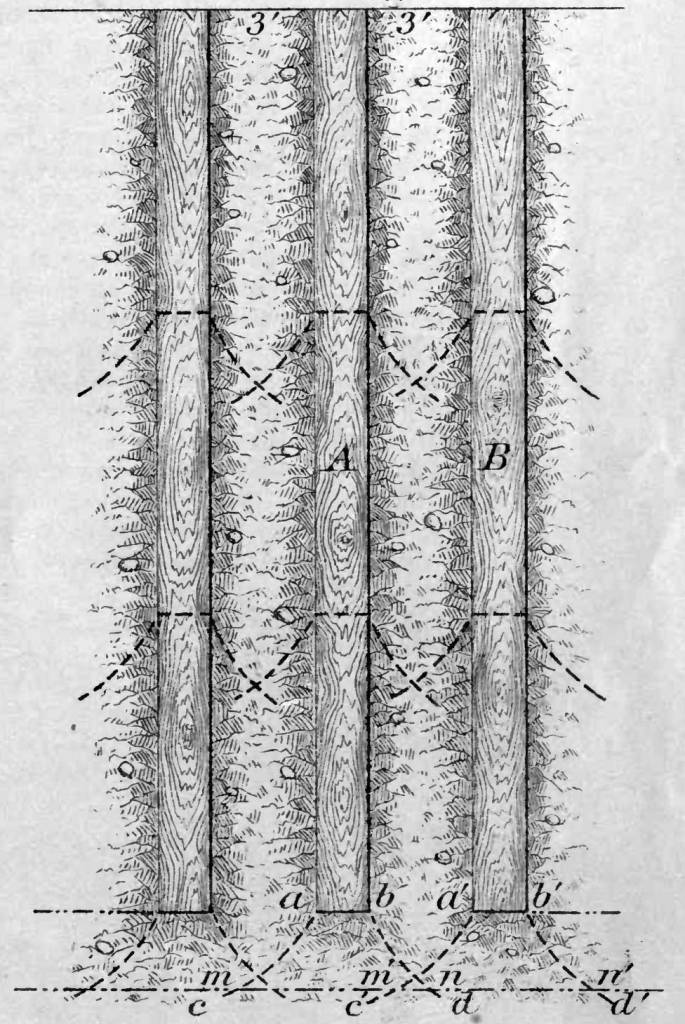
Let Figure 5 represent a plan of the piles of this foundation, and let Figure 6 represent a section through one of the rows. Let a, b, c, d, Figure 6, represent a section through the axis of the conoid of pressure arising from the pressure of the pile and its load, at the foot of the pile A, and let a’, b’, c’, d’, represent a similar section through the conoid of pressure at the foot of the pile B.

Let us pass a horizontal plane at any short distance say eighteen (18) inches below the feet of the piles which we suppose to be driven to a uniform depth), and let i, i, i, i and k, k, k, k, Figure 5, represent in plan, and let m, n, and m’, n’, represent in section, the areas cut from the conoids of pressure by this plane, and it will be seen that considerable portions of each of these areas, may be acted upon by pressures derived from both of the piles and their loads. The same may be said of the earth within the conoids of pressure surrounding the piles, and it appears therefore, that the forces acting upon the particles of earth below and surrounding a pile, may be in equilibrium, and the particles may be at rest, in the case of a loaded isolated pile, when the equilibrium may be disturbed, and the particles may sink with the pile, when the same load per pile is laid upon a foundation composed of piles driven in the same soil at such distances apart that their conoids of pressure intersect each other.

In the fine-grained soils of South Louisiana Elliot is qualitatively correct: the group capacity is less than the sum of the single pile capacity. Additionally in these types of soils the piles act as a “shallow foundation” and it is necessary to compute the consolidation settlement of the soft clays under that “foundation.” The construction of the fort was stopped in the spring of 1858 with the exhaustion of appropriation. When Weitzel returned to the site later that year, he observed a “marked settlement” of the fort, which was probably due to this consolidation. But that theory was also in the future as well. Subsequent to that inspection, as the report tersely noted, “The civil war also intervened,” and the “Federals” never completed the fortification.

Size Factor of Settlement

In addition to overseeing the fortification at Proctorsville, Beauregard also was in charge of building the New Orleans Custom House. Some of the formulae used to evaluate pile capacity relied on a maximum value of pressure on the pile head, and of course the resistance of shallow foundations to settlement are always of interest. Beauregard commissioned what amounted to an early “plate load test” to see what effect varying both the pressure and size of the foundation would have on the settlement.

The results for a single pressure are shown in Figure 7. The “square root of the foundation area” is of course the side dimension for a square foundation.

Although there are variations in the results, the general trend was correctly observed at the time: “It will be seen, by the above table, that, contrary to the general opinion, a larger surface sinks more in proportion to the area.” Although this principle underlies the extrapolation of the plate load test, and can be deduced from elastic theory, even in more recent times it bears repeating, as was evident in The Problem of Size: Gazetas and Stokoe (1991) Revisited.

An interesting variation was the 1” x 16” foundation. In current practice we would consider this a continuous foundation of 1” width, as the length is greater than 10 times the width, and design it as a 1” dimension foundation. Even as the square root of the area is 4”, the settlement was only 33”, which was low compared to some of the other results at that square root of area.

Conclusion

The Proctorsville project and its review by the Corps of Engineers demonstrated many of the weaknesses of the dynamic formulae, both in their underlying physics and in their factors of safety. It also touched on other aspects of foundation design which geotechnical research and practice would return to in the coming years. How one man responded to the challenge of the dynamic formulae, and how successful he was in solving the problem, is the subject of the next post.