The Case Method: An Overview and Worked Example

In my recent post Dynamic Measurement of Piles the Case Method was brought up and outlined. The Case Method is one of the oldest methods developed to estimate the static capacity of piles from dynamic measurements. The method is detailed in the FHWA document Design and Construction of Driven Pile Foundations; this will serve as an overview with a worked example.

The Basics

Instrumentation of pile behaviour during driving dates back to the 1930’s and the experiments of Glanville and his team, but today the normal way of instrumenting driven piles (and other deep foundations) for dynamic measurements is to attach a strain gauge and an accelerometer to the side of the pile just below the head. The strain gauge measures the compression (and a little tension) near the pile head and the computer to which the data is fed multiplies the strain by the Young’s Modulus of the pile material and the cross-sectional area of the pile head to yield the pile head force as a function of time. (The Young’s Modulus of steel piles is fairly straightforward; for concrete and wood things are a little more complicated, as this study showed.)

The acceleration-time curve is integrated to a velocity-time curve, as shown below.

It’s probably worth noting that we could make better predictions of soil resistance to driving (SRD) if we instrumented the pile at more than one place, but this method is relatively simple and economical to apply.

In any case, the Case Method is probably the easiest way of using this kind of data to estimate the SRD, and from an educational standpoint is the simplest to demonstrate the concepts of pile dynamics. It is based on several assumptions, the most important of which are as follows:

All of the soil resistance is concentrated at the pile toe.
The resistance at the toe is purely plastic, i.e., it does not have an elastic component.

The Method

The Case Method only requires that we know the following:

Force-time and velocity-time histories during ram impact on the pile;
Length of the pile;
Cross-sectional area of the pile head; and
Material properties of the pile, specifically its density and Young’s Modulus.

The basic equations of the Case Method is as follows:

$RTL = \frac{F1+F2}{2}+\frac{ZV1-ZV2}{2}$ (1)

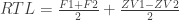
where

RTL = total resistance of the pile, both static and dynamic
F1 = pile head force at a time t₁
F2 = pile head force at a time t₂ = t₁ + (2L)/c
Z = pile head impedance. The concept of pile impedance is defined and discussed in Introduction to Wave Mechanics in Piling.
V1 = pile head velocity at a time t₁
V2 = pile head velocity at a time t₂ = t₁ + (2L)/c
L = length of pile
c = acoustic speed of pile material, also defined and discussed in Introduction to Wave Mechanics in Piling.

The static resistance (SRD) is then separated out by the equation

$RSP = RTL - J(ZV1 + F1 - RTL)$ (2)

where

RSP = static resistance of the pile
J = Case Damping Constant (dimensionless)

One question that may have arisen in your mind, in looking at the rather non-mathematically correct variables in Equations (1) and (2), is this: are the variables ZV1 and ZV2 simple scalars, or are they products of Z and V, thus $ZV1 = Z \times V1$ and $ZV2 = Z \times V2$ ? The answer is simple: both! If we multiply the velocity by the impedance, we get a force, and so we can plot the $Z \times V$ along with the forces. This is a key concept in pile dynamics. If we have a semi-infinite pile (i.e., a pile with a head but no toe) with no resistance along the shaft, $F = ZV$ . It is the finite nature of real piles, along with the effects of soil resistance, that makes pile dynamics possible.

Implementation and Example

One other thing we conveniently neglected to define were the times t₁ and t₂. The graphic below, from Design and Construction of Driven Pile Foundations, explains that for two variations of the Case Method, the RSP and RMX methods.

First: as explained earlier, t₂ = t₁ + (2L)/c always. The quantity (2L)/c is the time it takes for any part of the stress wave imparted by the impact of the hammer to make a full “round trip” down to the toe and back up to the head of the pile. Thus, the Case Method compares the same point in impact between two points where the same point in the stress wave has left the pile head and returned to the pile head.

That point is thus determined by t₁. That varies as follows:

RSP Method: t₁ takes place at the first peak of the force-time curve. The two peaks generally take place at the same time and, when the velocity is multiplied by the impedance, are generally the same or very close. This is because the movement of the pile hasn’t really started yet and thus hasn’t had a chance to affect the stress wave at the pile head. As noted in Design and Construction of Driven Pile Foundations, “The RSP or standard Case Method equation is best used to evaluate the nominal resistance of low displacement piles, and piles with large shaft resistances.”
RMX Method: t₁ takes place at a time 30 ms (typically) past the first peak of the force-time curve. As explained in Design and Construction of Driven Pile Foundations, “For displacement piles driven in soils with large toe quakes and for piles with large toe resistances, the maximum toe resistance is often delayed in time. This condition can be identified from the force and velocity records. In these instances, the standard Case Method equation may indicate a relatively low nominal resistance and the maximum Case Method equation, RMX, should be used.”

The examples above show how this is implemented in the same force-time and velocity-time histories for the two different methods. Note that the velocities are explicitly stated and then multiplied by the impedances to obtain ZV. In reality the entire velocity-time curves are multiplied by Z to enable them to be plotted along with the forces. It is not uncommon for the ZV plots to be presented “as is,” in which case it isn’t even necessary to know the pile impedance to compute Equations (1) and (2).

The Case Damping Constant

We’ve saved the “stickiest wicket” for last: the Case Damping Constant (J) itself. The two assumptions mentioned earlier have created problems for the Case Method, but the difficulties in evaluating the Case Damping Constant in advance of driving have presented the greatest challenge for the accuracy of the method.

This can be seen in the following table, from Design and Construction of Driven Pile Foundations:

It can be seen that there is quite a range for Case damping values, and it is also evident that the Case Method option (RSP or RMX) can affect the result. The core problem is that the Case damping is, strictly speaking, dependent upon the cross-sectional area of the pile in addition to the other, soil related variables. So, as is the case with the coefficient of subgrade reaction, there are size effects to consider as well.

However, if the method is to be used as a jobsite control technique and established by the actual conditions, the Case Method becomes potentially more useful.

Conclusion

The Case Method represented the first attempt at using dynamic data from impact pile driving to estimate the SRD of a pile. Although it has limitations and has been to a large extent superseded by methods such as CAPWAP, it can be useful in some situations. Additionally, it is very useful for teaching purposes to introduce students to pile dynamics, a subject that frequently gets inadequate coverage in undergraduate courses.