The Dennis and Olson Method for Determining the Static Capacity of Driven Piles

Don C. Warrington, PhD., P.E., University of Tennessee at Chattanooga
Orignal Date May 2011
Revised September 2017

Methods of estimating the static capacity of driven pile are almost as numerous as the dynamic formulae of years past. As was the case with dynamic formulae, some have become embedded in codes, standards and the literature.

All of these, however, need to be understood for what they are: estimates. These methods are necessary for at least a “first cut” in determining the ultimate capacity of a driven pile, be that for a wave equation analysis, the design of a structure, or whatever requirement. However, short of using generous factors of safety (ASD) or resistance factors (LRFD), these methods are usually not the “final word” in the ultimate capacity of driven pile foundations, either individual or group.

Many methods of static capacity estimate are very involved computationally, and include a great deal of theory. However, given the nature of the data engineers usually have to work with and the weaknesses in the application of many theories of mechanics of materials to soils (especially the theory of elasticity,) in most cases the computational effort is hardly worth it relative to the increase in accuracy.

The Dennis and Olson Method was developed in the early 1980’s by Roy Olson, now Professor Emeritus at the University of Texas at Austin (and a collaborator with Lymon Reese on many of his projects) and Norman Dennis, now Professor at the University of Arkansas (Dennis and Olson, 1983a and 1983b.) It was developed principally to estimate the axial ultimate capacity of steel pipe piles used in offshore platforms. The method can be used for both sands and clays, which is very important (many methods have only a sand or a clay version, and one has to mix methods for piles driven into a combination of the two.)

Overview of Driven Pile Design

The general equation for the ultimate axial capacity of driven piles is

Equation 1:

Where

Q = ultimate axial capacity of the pile, kN
Q_s = ultimate shaft capacity of the pile, kN
Q_t = ultimate toe capacity of the pile, kN
W_p = weight of the pile, kN

For piles loaded in compression, W_pis generally neglected because the toe capacity Q_t is a net toe capacity, and thus W_p is the difference between the weight of the pile and the weight of the soil it displaces, which is usually small. The capacity in compression is thus

Equation 2: (compression)

For tension piles,

Equation 3: (tension)

The shaft capacity is in turn estimated by the equation

Equation 4:

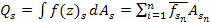
Where

f(z)_s = unit shaft friction along the pile shaft as a function of depth, kPa
A_s = shaft area of the pile which interfaces with the soil, m²
$\overline{f_{sn}}$ = average shaft friction along a portion n of the pile, kPa
$A_{sn}$ = shaft area of portion n of the pile, m²

Equation 4 is only solved in the integral form in theoretical considerations. For practical considerations, it is solved in the summation form. Piles are customarily divided up into regions with a reasonably uniform soil type and unit shaft resistance.

The capacity of the pile toe is computed by the equation

Equation 5:

Where

q_p = unit pile toe capacity, kPa
A_p = area of pile toe, m²

As mentioned earlier, one advantage of the Dennis and Olson method is that the method includes estimating the capacity of both sands and clays. We will consider each of these separately below, in turn considering both shaft and toe capacity for each soil type.

Capacity in Clays (Cohesive Soils)

Toe Capacity

The unit toe capacity in turn of piles in clay is given by the equation

Equation 6:

Where

c_u = undrained shear strength of the clay in the vicinity of the pile toe, kPa
F_c = correction factor for method of obtaining undrained shear strength
- = 0.7 for in situ vane shear tests
- = 1.1 for unconfined compression tests on sample of high quality
- = 1.8 for unconfined compression tests on samples taken with typical driven samplers
A_p = pile toe area, m²

Equation 6 is very similar to Tomlinson’s Method, a familiar method in FHWA publications.

There are two critical issues relating to Equation 6 that need to be considered:

Value of F_c: Dennis and Olson note that the values of F_ctabulated above are based on a very small database, and that it “should be larger for unconfined compression tests on stiff fissured and soft gaseous samples.” (Dennis and Olson (1981a), p. 384)
Pile plugging of open ended pipe piles. Most offshore pipe piles are driven open ended; plugging is an important issue with these piles. According to the authors, Equation 5 should be computed to be the smaller of one or two results:
1. The pile toe is analysed as if it were closed ended, which changes the way A_p is computed.
2. The toe capacity is the sum of the result of Equation 5 (with A_p being the cross-sectional area of an open-ended pile) and the shaft capacity of a pile plug which extends the full length the pile is embedded in the soil.

It should be noted that, since the method was formulated, a good deal of research on plugging of open-ended pipe piles and H-beams has been done. Some of this is summarised in Hannigan et. al. (1997).

Shaft Capacity

The equation for the unit shaft capacity at a given point or region along the pile shaft is

Equation 7:

Where

α = adhesion factor
$\overline{c_u}$ = average undrained shear strength over a segment (or the entire length) of the pile, kPa
F_L = correction factor for pile penetration

Values for α are given in tabular form in Table 1 and in graphical form in Figure 1. These values are meant to be interpolated, as is clear from the graph.

Table 1 Values for c_uF_cvs. α

c_uF_c, ksf	c_uF_c, kPa	α
0	0	1
0.6	30	1
1.2	60	0.5
5	240	0.3
∞	∞	0.3

Figure 1 Values for c_uF_cvs. α

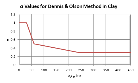
Note that the dependent variable is a product of the undrained shear strength and the soil strength correction factor.

The correlation for α is similar in concept to the familiar API method, but is more conservative. The authors adopted the use of an α-method for simplicity. The authors note that the method was developed from data on normally or lightly overconsolidated clays and may not be applicable for other soil conditions.

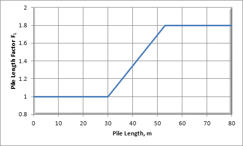
The pile penetration factor is given in a similar manner, in tabular form in Table 2 and in graphical form in Figure 2.

Table 2 Values of F_L vs. L

L, ft.	L, m	F_L
0	0	1
100	30	1
175	53	1.8
250	80	1.8

Figure 2 Values for Pile Length L vs. F_L

Capacity in Sand (Cohesionless Soils)

Toe Capacity

As is the case with most static pile capacity methods, the Dennis and Olson Method uses a bearing capacity type of equation for the toe capacity, analogous to shallow foundations. The method modifies this a bit as follows:

Equation 8:

Where

σ_vo = effective stress at the pile toe, kPa
N_q = bearing capacity factor (see Table 3.)

Table 3 Values of δ and N_q

Soil Description	δ	N_q
*Very Loose Siliceous Sand, Medium Silt, Loose-Medium Calcareous Sand, or Medium Sandy Silt**	15	8
*Dense Silt, Silty Sand, Medium-Dense Calcareous Sand, or Loose Siliceous Sand**	20	12
Dense Sandy Silt, Medium Siliceous Sand or Medium Silty Sand	25	20
Dense Siliceous Sand or Very Dense Silty Sand	30	40
Very Dense Siliceous Sand or Dense Gravel	35	50

* Calcareous sand is defined as consisting of at least 90% calcium carbonate.

Shaft Resistance

As is the case with cohesionless soils, the strength of the soil is developed by the effective stress. The unit shaft resistance in a cohesionless layer is given by the equation

Equation 9:

Where

and

K = lateral earth pressure coefficient = 0.8 if values for δ given in Table 3 are used
D = depth of the centre of the layer, m (use consistent units in any case)
B = diameter of the pile, m (use consistent units in any case)
δ = angle of friction between the pile and the soil (see Table 3.)

Example of the Method

Consider the pile shown in Figure 3.

Figure 3 Example Problem for Dennis and Olson Method

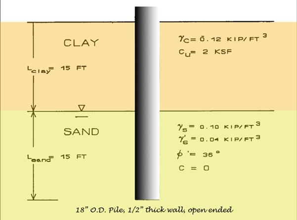
Let us determine the ultimate pile capacity (tension and compression) using the Dennis and Olson method. Since the pile is open ended, there is a possibility that it will plug. Although there are newer methods of evaluating plugging, for simplicity’s sake we will use the method’s own criterion, as stated earlier. Also assume that the values of c_u for the clay layer were obtained from in situ vane shear tests.

The first thing we need to do is to construct a “P_o” diagram of the effective stresses of the soil. The P_o diagram for this profile is shown in Figure 4.

Figure 4 P_o (Effective Stress) Diagram for Sample Soil Profile

The important points are as follows:

Effective Stress at Clay/Sand Layer Boundary = 1800 psf
Average Effective Stress in Clay Layer = 900 psf
Effective Stress at Pile Toe = 2400 psf
Average Effective Stress in Sand Layer = 2100 psf

We proceed to analyse the system using the equations given. From Equation 1, the weight of the pile is

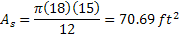
Turning to Equation 4, we need first to compute the whetted shaft area for each layer. Since the pile is uniform and the layers are the same thickness, the areas are the same, thus

The unit shaft capacity for the clay layer is given by Equation 7. From the problem statement, F_c = 0.7, thus c_uF_c = (0.7)(2) = 1.4 ksf. Since 1.2 < c_uF_c < 5, α will have to be determined by linear interpolation. From Table 1, α = 0.49. Substituting these values, we have

For the sand layer, the unit shaft capacity is given by Equation 9. The centre of the layer is 22.5’, and so F_SD = (5/3)e^{(-1.5/((60)(22.5))} = 1.66. From previous considerations, σ_vo = 2100 psf and K = 0.8. Based on the unit weight data of the soil, we have a very loose sand in this layer, so from Table 3 δ = 15˚. Substituting, we have

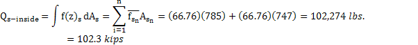
The total shaft resistance, from Equation 4, is

We can see from this that, as is typically the case with driven piles, the weight of the pile is very small relative to the shaft capacity, let alone the total ultimate capacity of the pile.

Turning to the pile toe, since the pile toe is in sand Equation 8 applies. For the toe, F_D = 1/(0.15 + (0.08)(30)) = 0.39, σ_vo = 2400 psf and N_q = 8 (from Table 3.) Substituting,

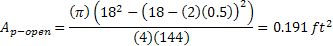
Since plugging is possible, we must compute the toe areas of both an open and closed ended pipe pile. For the open end, A_t is

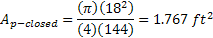
And for the closed end

With the plugging options, Option 2a gives the following toe resistance (Equation 5):

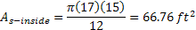
Option 2b is somewhat more complicated to compute because of the inner shaft resistance; however, since we have computed all of the unit shaft resistances, the most difficult task is done. The inner wetted soil surfaces for the two layers are, using an inside diameter of 17”,

In a similar manner to the outside shaft resistance, the inside shaft resistance is computed as follows:

The toe capacity for an open ended pile is

Therefore

Obviously Q_pa < Q_pb, so Q_p = 13.3 kips. Again, for a newer and more thorough treatment of plugging, see Hannigan et. al. (1997).

From this, the ultimate capacity of the pile in compression (Equation 2) is

And the ultimate capacity of the pile in tension (Equation 3) is

Notes about the Method

The selection of the “F” factors for both sand and clay is critical to obtain proper results. For example, the selection of F_c can vary the working undrained shear strength by more than a factor of two.
A more updated analysis of pile plugging than the method proposed is probably in order, at least as another alternative to compute the toe resistance. In the case of this problem, Hannigan et. al. (1997) suggest that the aspect ratio of the pile (L/B) is just large enough to initiate plugging; therefore, a more reasonable approach may be to compute the toe resistance as the product of the unit toe resistance and the toe area of an open-ended pile (the cross-sectional area of the pile, as it is uniform.)

Conclusion

The Dennis and Olson Method is a simple method of determining the axial capacity of driven piles in either sand, clay or (as shown above) a combination of both. It avoids the complexities of methods which are more closely based on theory. In the case of clays, it is also more conservative than the widely used API method.

References

DENNIS, N.D, and OLSON, R.E. (1983a) “Axial Capacity of Steel Pipe Piles in Clay.” Proceedings of the Conference on Geotechnical Practice on Offshore Engineering, pp. 370-388. New York: American Society of Civil Engineers.

DENNIS, N.D, and OLSON, R.E. (1983b) “Axial Capacity of Steel Pipe Piles in Sand.” Proceedings of the Conference on Geotechnical Practice on Offshore Engineering, pp. 389-402. New York: American Society of Civil Engineers.

HANNIGAN, P.J., GOBLE, G.G., THENDEAN, G., LIKINS, G.E. and RAUSCHE, F. (1997) Design and Construction of Driven Pile Foundations. FHWA HI 97-103, 2 Volumes. Washington, DC: Federal Highway Administration.