
It’s my custom to review papers which cite my own work. This pair of papers, whose lead author is Tu Yuan from Zhejiang Sci-Tech University in Hangzhou, China, is interesting because it take an approach whose basic concept goes back a long way in pile dynamics and which needed some basic advancement.
The two papers can be found from here:
- Nonlinear fictitious-soil pile model for pile high-strain dynamic analysis
- Fictitious soil pile model for dynamic analysis of pipe piles under high strain conditions
The abstract for the first one is as follows:
Existing numerical models for simulating the pile behaviours in high-strain dynamic load tests (DLTs) cannot account for the wave propagation in base soil. This paper proposes a nonlinear fictitious-soil pile (FSP) model to better simulate the base soil. The proposed model regards the base soil as a FSP with a cone angle extending from pile toe to bedrock, and simulates shaft resistance by improved Randolph model. The pile-soil system is discretized into a series of mass-nonlinear springs, and was solved based on the Newmark’s β method. The proposed model was validated by comparing its predictions with those obtained from Randolph model and Smith model, as well as field measurements of driven and bored piles in different sites. Parametric study demonstrated that the calculated results were significantly affected by the discretization degree, FSP dimensions and soil nonlinearity. The displacement attenuation in base soil is nonlinear, and the impact energy is consumed rapidly near pile toe. Besides, large-diameter piles tend to have a larger affected zone, in which the wave phenomenon in base soil should be considered. Empirical formulas for soil affected zone and required pile displacements in DLTs were proposed to facilitate the practical application of FSP model.
The paper of mine both cite is the ZWAVE paper, which I presented in 1988. They did so because of my use of Randolph and Simons (1986) model for the soil around a pile during driving. At the time I felt that a soil model that was based on the properties of the actual soil made more sense than something which did not, such as Smith (1960). Getting to such a correlation is easier said than done, and raises a question that has been in front of the profession since the dawn of pile dynamics: how is it possible to properly model the soil response, the soil being a 3D continuum around the pile, with 1D or 2D methods?
Since the ZWAVE paper I have done some further work on this topic, some of which relates to the subject matter at hand.
The first is Improved Methods for Forward and Inverse Solution of the Wave Equation for Piles, where I actually developed a 3D (really, a 2D axisymmetric model) to model the pile-hammer-soil system during driving. This technique has become more common, especially for static applications. I am still of the conviction that something like this is where we’re going to end up. However, getting past the institutional inertia may be as big or a bigger challenge than to get a model which can be shown to work. We also have to deal with the fact that pile driving is a “continuous” process and changes to the soil during that driving are significant in the performance of the system, as noted in Comments on “A novel soil reaction model for continuous impact pile driving.”
The second is Estimating Load-Deflection Characteristics for the Shaft Resistance of Piles Using Hyperbolic Strain Softening. Randolph and Simons’ model was an outgrowth of their elastic modelling of pile deflections under load; this considers the effect of strain softening. The result suggested that the deflection-related soil response, all things taken into consideration, is still linear, although the coefficients we use may require some modification.
The third–and the most important relative to the present works under discussion–is the modelling of the soil under the pile toe. The papers present a model which basically constructs a “fictitious” pile made up of soil under the toe, as opposed to trying to model the dynamic toe resistance by a single, discrete system, as is customary with most current wave equation models, by a truncated cone divided into elements. The difference between the two is that the first one uses a soiid truncated cone; the second divides the cone into an inner cylinder under the hollow of an open-ended pipe pile and an outer truncated cone with the rest of the material.
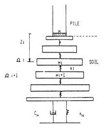
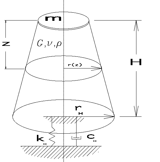
This issue came up in my Closed Form Solution of the Wave Equation for Piles, albeit for a different reason. In the course of modelling the pile toe in closed form, I drew from the researches of Alain Holeyman, who is one of the best academics in the driven pile field, both impact and vibratory. The paper which influenced my thinking on this was his “Unidimensional modellization of dynamic footing behaviour,” from the Proceedings of the International Symposium on Penetrability and Drivability of Piles, San Francisco, 10 August 1985. Tokyo: Japanese Society of Soil Mechanics and Foundation Engineering. A diagram of his model under the pile toe can be seen at the right.

A diagram of my interpretation of that for my thesis is on the left.
Obviously the current authors have taken this to a higher level. The advantage of such a model–especially when done discretely, as Holeyman and the authors of the present works show–is that the 1D model can simply be appended to the pile toe. In the case of adding the soil plug, things get a little more complicated but what we end up with is two 1D systems that interact with each other.
I will remind my readers that the whole business of modelling the pile toe–especially as it related to the pile toe quake–has been one of the most uncertain aspects of wave equation modelling for a long time.
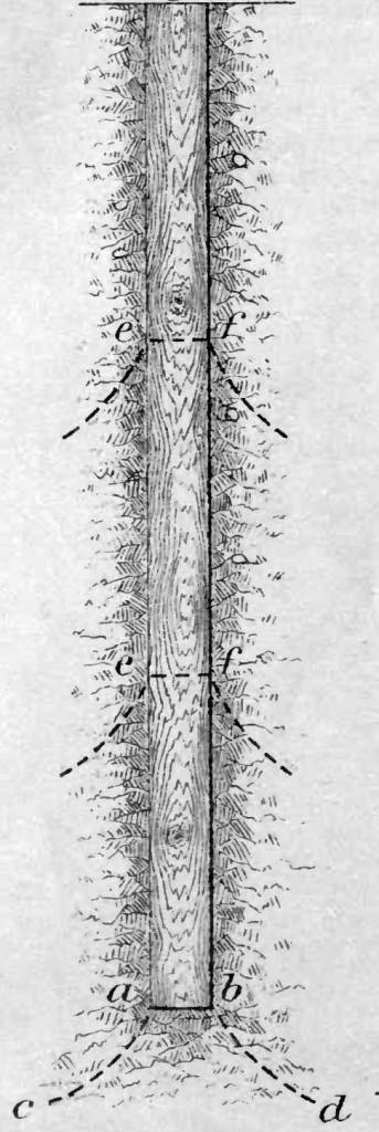
I think it’s also worthwhile to take a trip back in time and look at my last post: Putting Dynamic Formulae to the Test: the Proctorsville Fort Project. This project, started but not finished in 1856-8 and documented with analysis in 1881–delved into two issues, albeit in an unadvanced state, which bear on the present two papers.
The first was that these researchers posited that the pile toe response was in a “conoidal” region, i.e., the truncated cone of the present papers. Subsequent to that researchers focused on the pile toe as a sort of shallow foundation that could be modelled using bearing capacity considerations, but the depth of the pile toe is such that shallow foundation bearing capacity has some significant limitations in modelling the pile toe, either statically or dynamically.
The second included speculation on how much of the soil moved during driving and was thus involved in the driving system. This also appears in Goodrich (1908). Solving this problem is, of course, core to any 1D representation of pile driving, and although we have made many advances since these early times we still have some ways to go.
“The thing that hath been, it is that which shall be; and that which is done is that which shall be done: and there is no new thing under the sun.” (Ecclesiastes 1:9)
“In any investigation such as this the ideal goal is to come up with something truly novel, and many of such works emphasize their novelty to the denigration of those who have gone on before. While in some fields of endeavour this might be appropriate, in this case such sweeping novelty cannot be claimed. This work fits the mould as outlined by Pascal above: it takes the work that has been done before, advances it a step while realizing that there are many more steps before “perfection” is achieved.” Closed Form Solution of the Wave Equation for Piles


One thought on “Comments on “Nonlinear fictitious-soil pile model for pile high-strain dynamic analysis” and “Fictitious soil pile model for dynamic analysis of pipe piles under high strain conditions””