
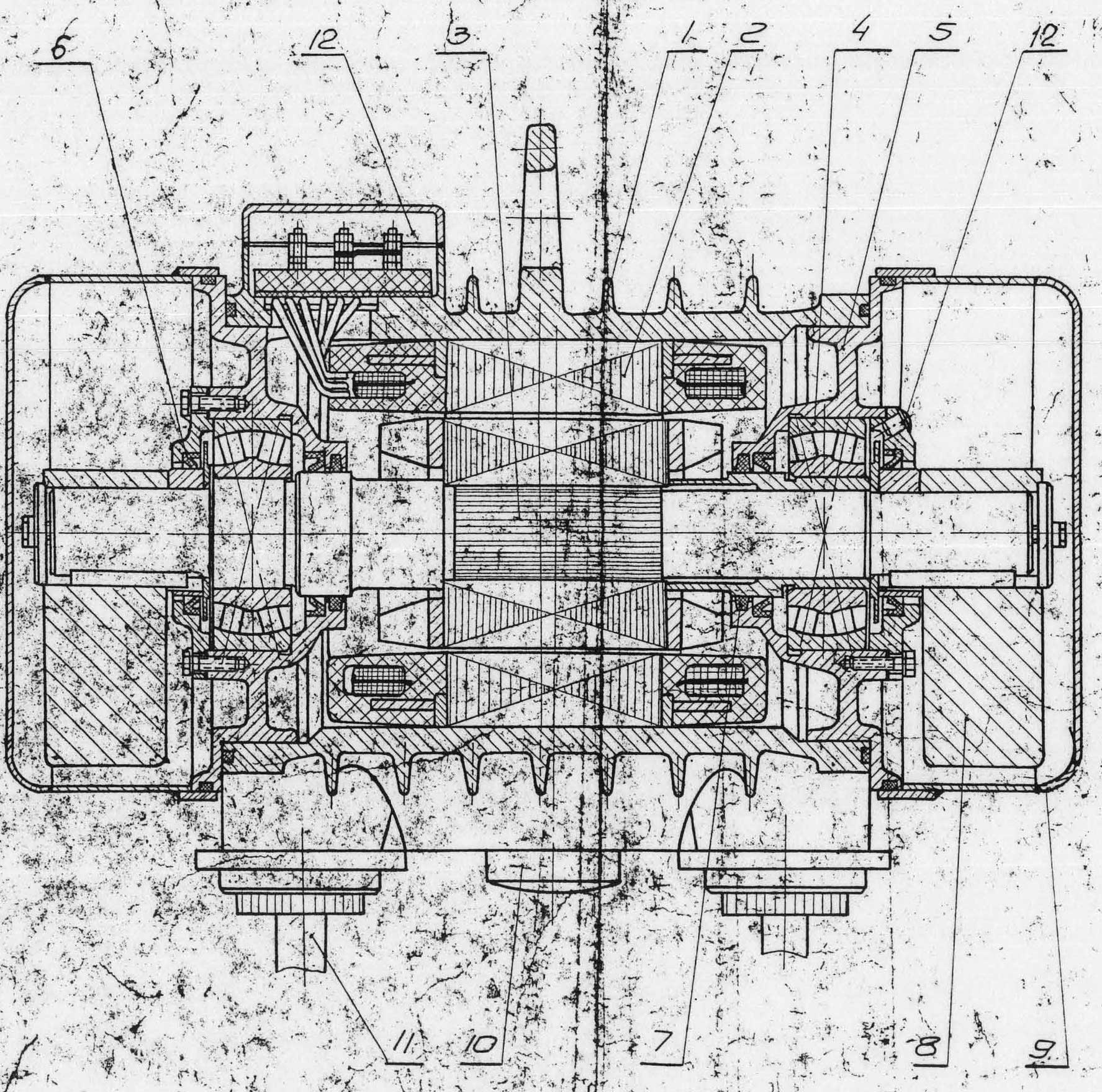
In my earlier post Checking the Soviets: Determining the Bending of the Shaft, I went into the analysis of the centre shaft of the machine. For my Statics course at Lee University, I want to go through a “hand” analysis of this. The machine is shown above. A simpler drawing of the shaft itself is shown below.

Let’s first look at the basic loading diagram, shown below.
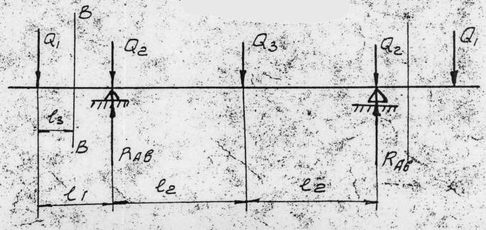
The geometry and loads are defined as follows:
- Length l1 = 9.2 cm (same on both ends)
- Length l2 = 19 cm
- Load Q1 = 44.15 kN
- Load Q2 = 4.415 kN
- Load Q3 = 32.37 kN
A beam diagram (from the CFRAME finite element program) showing the supports and loading points is shown below.

Note that, as usual, we have one support (the left one) that is constrained in the x- and y-directions and the other (the right one) that is only constrained in the y-direction. Both are free to rotate. This is to prevent static indeterminacy due to shortening of the beam in bending.
Our goal is to determine the bending moments at Points 2 and 3 on the diagram above.
This is a loading diagram (the loads are in Newtons):

There are two ways of determining the reactions. The first is the formal way, i.e., taking moments around one of the reactions. Let’s do it around the left bearing (Point 2); the summation of moments is as follows (the forces at Point 2 have no effect because they have a zero moment arm):
-(44.15 kN)(9.2 cm) + (32.37 kN)(19 cm) + (4.415)(38 cm) + (RAB) (38 cm) + (44.15 kN)(47.2 cm) = 0 (1)
Solving, RAB = −64.75 kN.
It should be evident that, by symmetry, both reactions are the same. But that leads us to the second solution: simply taking all of the loads, summing them up, and then dividing them by two to obtain the reactions. The sum of the loads is 129.5 kN; dividing this by two gives the same result, but in the opposite direction to maintain static equilibrium
Turning to the moment at Point 2, starting at point 1 and moving right, is it simply
-(44.15 kN)(9.2 cm) + (64.75 kN) (0) = 406.1 kN-cm. (2)
For Point 3, again starting at Point 1 and moving through Point 2, we have
-(44.15 kN)(28.2 cm) + (64.75 kN) (19) – (4.415)(19 cm) = 98.59 kN-cm (3)
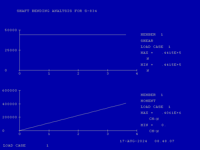
Now let’s turn to the shear and moment diagrams. As I did earlier, I’ll use CFRAME to do my drawing. The shear diagram for the entire shaft is shown below.

If you look at the hand-drawn diagram at the start of the post, you’ll see an “l3” length from the left end of the shaft. That’s used to draw the shear and moment diagrams. With only point loads, the shear in the Shaft Segment 1 (from Points 1 to 2) is a constant and is simply the value of Q1. (Draw a free-body diagram to show that this is the case.) The equation for shear in Shaft Segment 1 is
V = 44.15 kN (4, Shaft Segment 1)
If we integrate this with respect to x, for the moment we get
M = 44.15 l3, kN-cm (5, Shaft Segment 1)
You can see what these look like in the shear and moment diagrams below. You can also see that the moment at the reaction is the same as computed in Equation (2). (Frankly I’m not sure what’s going on with the scaling of the x-axis in this graphic; I think it’s in inches.)
Turning to Shaft Segment 2 (Points 2-3,) things are a little trickier since we don’t start at the origin but at x = 9.2 cm. The shear in this segment is
V = Q1 + Q2 – RAB = 44.15 + 4.415 – 64.75 = −16.185 kN (4, Shaft Segment 2)
The moment is had by integration, which is
M = -16.85 x + C (4a, Shaft Segment 2)
If we substitute M = 406.1 kN-cm and x = 9.2 and Point 2, we solve for the constant, and the moment equation becomes
M = -16.85 x + 555.002 (5, Shaft Segment 2)
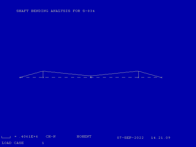
The shear and moment diagrams for Shaft Section 2 are below.

The moment for the end points at 9.2 and 28.2 cm can be checked and compared with the results above. Since the shaft is symmetric about the centre point, the results for the right side of the shaft are mirrored of those on the left, as can be seen from the shear diagram earlier and the moment diagram below.
Shear and moment diagrams for point loads are fairly straightforward. Those for distributed loads (which are very common in places like retaining walls and laterally loaded piles) can be another matter altogether, as can be seen in Designing Cantilever Sheet Pile Walls Using a Chart.
Appendix: Determining the Moments Using a Distributed Load of the Shaft Itself
The original designers included the effect of the decelerating shaft by incorporating them in two of the point loads: Q2 (entirely the shaft) and Q3 (partially the shaft.) So how would the analysis–and the results–be different if the shaft load were distributed across the entire length of the shaft?
Let us begin by assuming the shaft is a solid uniform cylinder with a diameter of 6.2 cm. The cross-sectional area of the shaft is 30.191 cm2. Assuming the weight of the shaft is 7.8 g/cm3, the mass of the shaft per linear centimeter is (30.191)(7.8) = 235.4898 g/cm = 0.2354898 kg/cm. The weight of the shaft per linear centimeter is (0.2354898)(9.8) = 2.3078 N/cm. For a design deceleration of 150 g’s, the distributed load on the shaft is (2.3078)(150) = 346.2 N/cm = .3462 kN/cm.
Now we must deduct the shaft load from the point loads Q2 and Q3. The shaft is 56.4 cm long, so the total inertial load of the shaft is (.3462)(56.4) = 19.524 KN. We first subtract all of the Q2 loads from this, or 19.524 – (2)(4.415 N) = 10.694 kN. We then subtract this from Q3 to obtain a new Q3‘ = 32.37 – 10.694 = 21.68 kN, the new Q2‘ = 0.
This new load case is illustrated in the diagram below, the loads in N and N/cm.

At this point we need to determine the reactions. We have the same decision as with the purely point load case above: do we take moments about one support or do we simply use symmetry? To take the moments, we would need to backtrack through some of our calculations and concentrate the distributed loads on the segments before taking moments. It should be evident that the simpler approach would be to use symmetry and add up all the loads (point and distributed) and divide them evenly between the two supports. Doing this yields the same result as we had before, i.e., RAB = −64.75 kN. This is also a good check on whether we distributed the shaft load properly. This is also crucial in constructing the shear and moment diagrams properly.
This done, let us proceed by considering the shear and moment diagrams for Shaft Segment 1 (Points 1 and 2.) The shear is given as
V = 44.15 + .3462 x (6a, Shaft Segment 1)
Integrating to the moment,
M = .3462x2/2 + 44.15 x (6b, Shaft Segment 1)
The integration constant is zero because, at x = 0, M = 0. At Point 2 (x = 9.2 cm), the moment is 42.08 kN-cm, as shown below.
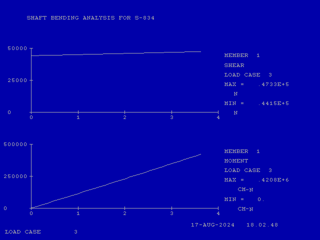
If we compare the shear diagram with the previous case, we see that it is flat for the previous case and only slightly sloped upward for this case. The distribution of the shaft resistance is not really that different, but it does result in a moment at the bearing that is about 4% greater than the original calculation.
Turning to the Shaft Segment 2 (Points 2 and 3,) the shear can be expressed as follows:
V = .3462 (x – 9.2) -17.42 = .3462 x – 20.61 (6a, Shaft Segment 2)
The second term -17.42 is the shear at the support at x = 9.2 cm. Integrating,
M = .3462x2/2 -20.61 x + C (6b, Shaft Segment 2)
The constant can be found by substituting x = 9.2 and M = 42.08 kN-cm, thus C = 217.04 kN-cm. The results are plotted below.
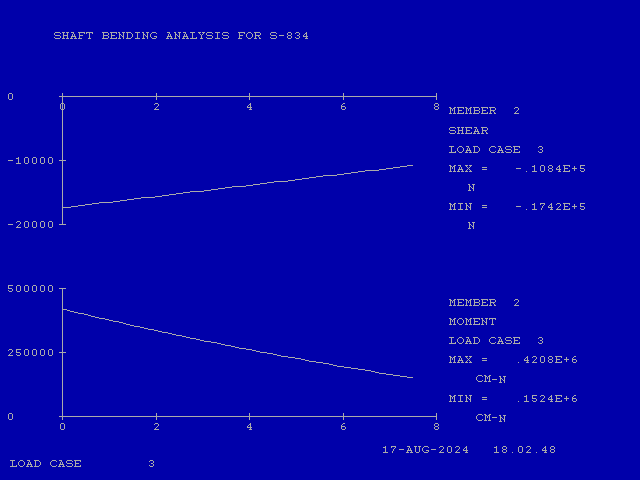
The effect of the distributed load on the shear and moment are more pronounced than in Shaft Segment 1, but this is because this segment is almost twice as long as that segment. The moment at Point 3 has increased to 15.24 kN-cm from 9.859 kN-cm, a 55% increase (although this point is not the maximum moment on the shaft.)
The shear and moment diagrams for the whole shaft (which again is symmetric) with the distributed load are shown below.

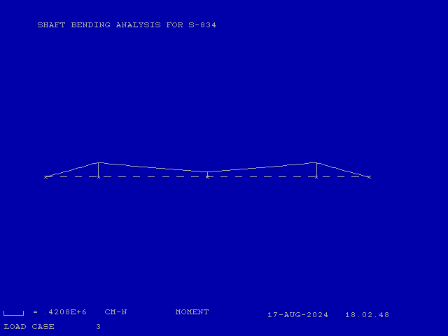
Although it is likely the shaft design would have changed little, applying a truly distributed load can change the shear and moment results for a beam substantially, in this case with little additional computational effort.


One thought on ““Hand” Solution for the Centre Shaft for the S-834 Impact-Vibration Hammer”