Driven Pile Design: Static Load Testing and Axial Settlement

In the previous post we looked at the various ways of computing the “bearing capacity” of the pile. We also made the case that “bearing capacity” wasn’t a really accurate way of characterising the load bearing performance of a driven pile. In this post we will address both of these issues and show the most comprehensive way that load bearing performance can be characterised, and the means by which we test for it.

More Resources

• Foundation Design and Analysis: Deep Foundations, Static Load Testing
• Foundation Design and Analysis: Deep Foundations, Driven Pile Settlement and Group Capacity
• Design and Construction of Driven Pile Foundations, 2016 Edition, Volume II covers the topics discussed in this post.

Static Load Testing

Static load testing is the “gold standard” of determining the load-settlement characteristics of a deep foundation. You can find details of it in the publication Static Testing of Deep Foundations. The following is a brief overview of static load testing and its interpretation. It is generally conducted in accordance with ASTM D1143.

Static load testing involves the application of a stepwise load at the head of the pile. This results in a load-settlement curve such as those seen on the right. How the load-settlement curve is shaped depends upon a) the type of soil(s) that the pile is driven into, and b) the way in which the soil resistance is divided between the shaft and the toe. The pile itself experiences elastic compression during loading and this too contributes to the settlement of the pile.

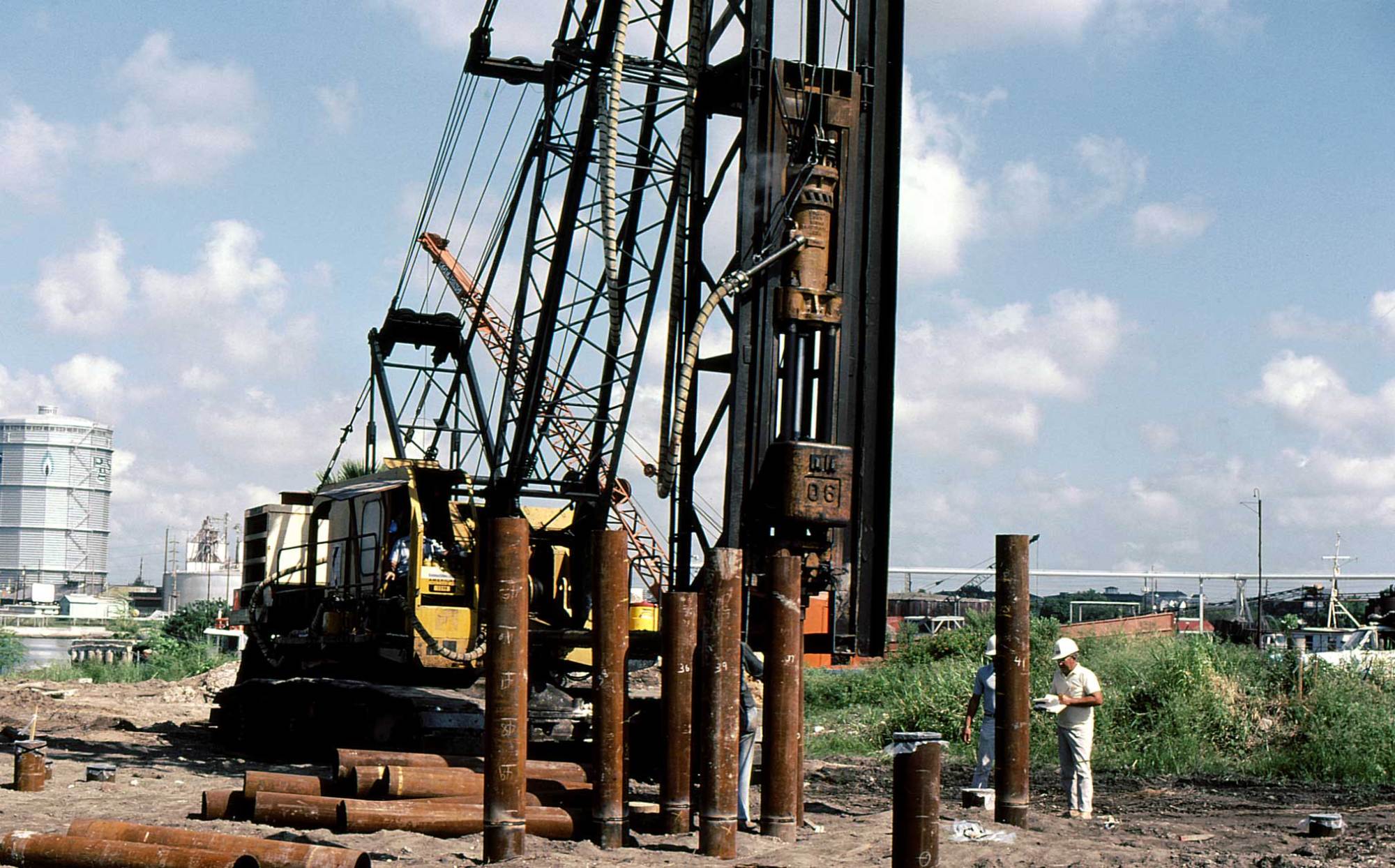
Although one might think initially that a large dead weight be applied to the pile head, in reality most static load testing is done using a reaction system and beam, where there are two adjacent piles joined by a beam against which the load is applied using a jack, as shown below.

Having a load-settlement curve is interesting, especially with deflection-sensitive foundations, but that leads to the next question: how does one extract a “bearing capacity” or ultimate load from a static load test. As we see below, the answer is not obvious; there is more than one way to interpret a static load test.

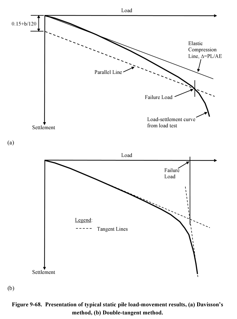
These are just two methods; there are more, as is illustrated at the left. For the load-settlement calculations we will be doing, we will use Davisson’s Method. It is an “offset-yield” method similar to those used with metals and is outlined below (from NAVFAC DM 7.02.) The purpose of arriving at this number is not to bypass the settlement issue but to establish a load beyond which plunging failure becomes a real possibility.

Methods of Estimating Settlement

As is the case with so many geotechnical problems, settlement of driven piles is a very nonlinear problem. There have been “closed form” solutions over the year; one of those will be presented here. With the technology we have the best way to solve the problem is to use a computer solution, and the most common of those are so-called “t-z” solutions.

T-Z Solutions

A diagram of a t-z solution is shown at the right. The pile is divided up into segments and the response of the soil to pile movement is modelled in the springs. The springs can be non-linear (as shown in the diagram) or piecewise linear. The toe is similarly modelled.

As is the case with static load testing, the load P_o is applied stepwise and a load-settlement curve is developed that (hopefully) will resemble a static load test, and in the case of matching a static load test, the parameters can be adjusted so that there is a match.

PX4C3

There are many programs that have been developed over the year to address this problem. The one we will use here is PX4C3, developed in the early 1970’s by Lymon Reese and Harry Coyle. It is very rudimentary (in its current state it is only really useful on open-ended pipe piles, which is what we have here) but works fairly well. The documentation for the program–along with the program itself–can be found here. The program was used “as is” and the data file was assembled by hand. The following should be noted in the assembly of the data to run the program:

• The capacities from the Fellenius Method were used to determine the maximum shaft and toe resistances. The four-layer division was used, hopefully it made for a more accurate result.
• Although it would have been simpler to use an elastic-purely plastic model, the curves from that kind of model tend to be unrealistically “blocky.” PX4C3 has a very flexible input for different kinds of load transfer curves for different consistency and types of soils. For this analysis the load transfer model of Vijayvergiya (1977) was used. It is simple to implement and the application to both cohesionless and cohesive soils is very similar. This is outlined in Mosher and Dawkins (2000) but a few things got “lost in the translation” and with other assumptions the method was implemented as follows:
  • The quake w_c for all shaft friction was set at 0.25″.
  • In Vijayvergiya’s original paper the inverse exponent for the load-transfer curve at the toe was N=3, this is what was used here.
  • Vijayvergiya in his original paper the quake z_c for toe stated that “An average range of z_c from 0.04B to 0.06B may be used for both sand and clay, where B is the pile tip diameter or width.” A value of 0.05B was used; in this case this works out to z_c = (0.05)(18) = 0.9″.

The normalised t-z curves for the shaft and toe resistances for this specific problem are shown below.

The graphical results will be shown below along with Davisson’s and Vesić’s method. The calculations, graphs and input data for all of these can be seen along with the spreadsheet solution for Fellenius’ Method.

Vesić’s Method

This is probably the simplest method of estimating the settlement of either driven or drilled piles. There is a complete explanation of it here with a worked example. It will not be repeated here, but the calculations for this particular pile and case are presented in spreadsheet form here. Most of the parameters are similar to those for PX4C3; however, the value for C_s = 0.03 from the table of recommended values.

Comparison

A graphical comparison of the two methods and Davisson’s interpretation of them are presented below.

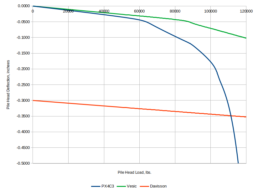
Some comments are as follows:

• The result from PX4C3 looks reasonable, like it came from a static load test.
• The Davisson line crosses the PX4C3 line at about 110 kips, which is the Davisson load.
• The deflection result from Vesić’s Method is unrealistically low. The main problem is that the recommended value for C_s is doubtless low by a factor of at least four, which would be more in the range of bored piles. As mentioned before, the soil properties are not internally consistent. Compounding the problem is the fact that 30′ is too short for most 18″ diameter driven piles; the pile is “stiff,” which explains the flat Davisson line. A more realistic example of this is given in the post Vesić’s Method of Estimating the Settlement of Driven Piles and Drilled Shafts.

References

• Vijayvergiya, V. N. (1977). “Load-movement characteristics of piles,” Proceedings, Ports 77, American Society of Civil Engineers, Vol II, 269-286.