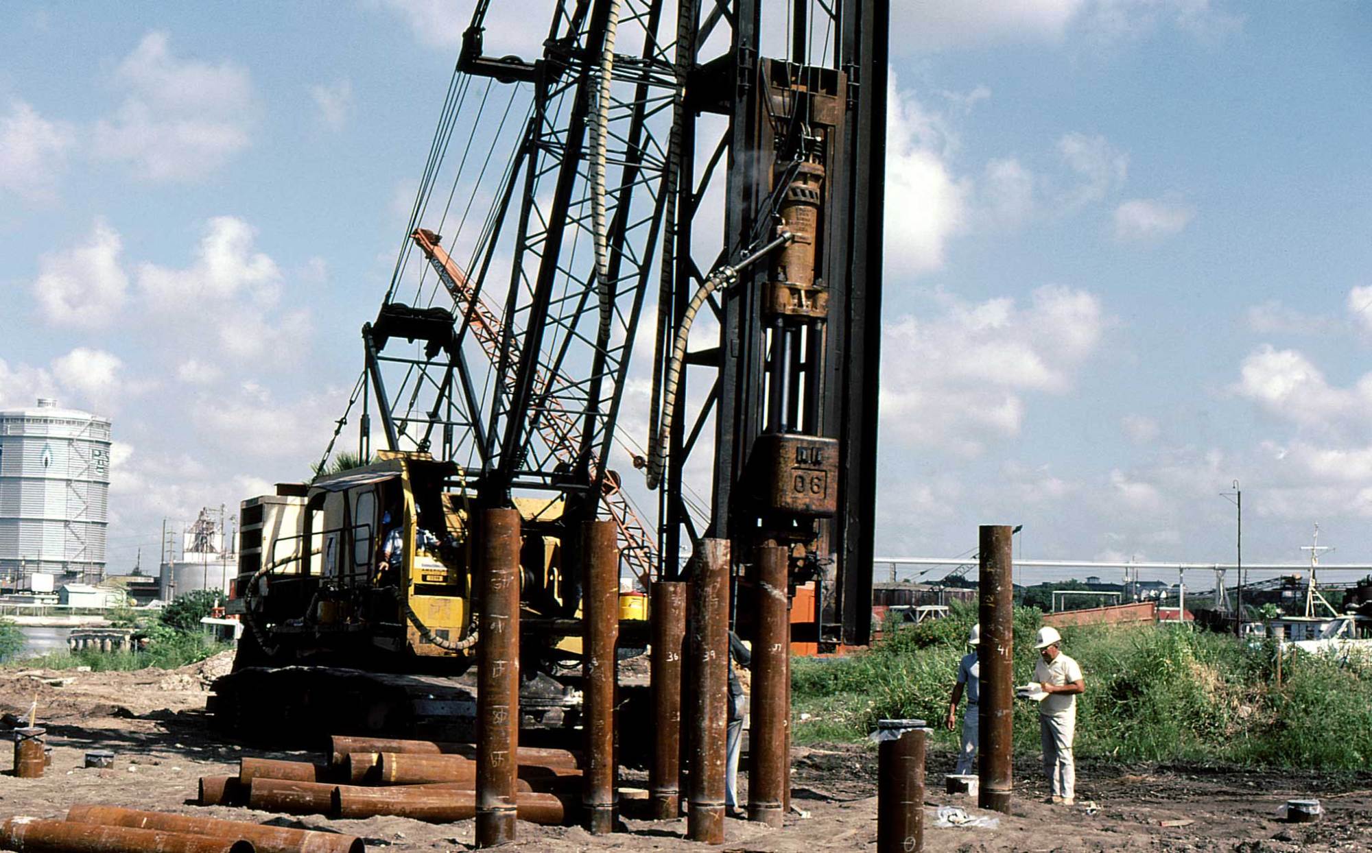
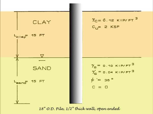
Driven Pile Design: Three Methods of Analysis

As mentioned earlier, it would be a long business to catalog all of the methods that have been devised to estimate the axial bearing capacity (with all of the problems of that concept) of driven piles. Here we will show how three of these methods apply to our test case (reproduced below.)

More Resources

Foundation Design and Analysis: Deep Foundations, Driven Pile Bearing Capacity
Finno, R.J, Editor (1989). Predicted and Observed Axial Behavior of Piles: Results of a Pile Prediction Symposium, American Society of Civil Engineers, New York, NY. An interesting study where a large number of these methods were tested against actual results.
Design and Construction of Driven Pile Foundations, 2016 Edition, Volume I covers the topics discussed in this post.

Soil Plugging

One of the knottiest problems with open ended pipe piles (which we have here) is the issue of soil plugging. A diagram of the phenomenon is shown at the right. As the pile advances, under certain conditions soil will advance on the inside of the pile, which changes both the toe resistance and, for the lower reaches of the pile, the shaft resistance as well. Predicting and modelling this phenomenon has been one of the challenges of driven pile design and is beyond the scope of this series. It is noteworthy that one of the early ways of dealing with this problem is to model the toe as a closed ended (also shown in the diagram.) This is enshrined in an option to the Dennis and Olson Method, and although it may seem obsolete I have seen recent (2024) drivability analyses where it is still practiced.

It’s also worth noting that H-piles are subject to plugging, and also worth noting that the shaft perimeter of an H-pile can either be the whole perimeter or the perimeter of the flanges and the plug (more conservative.) Some information on that topic is shown at the left, and further discussion of it is at Foundation Design and Analysis: Deep Foundations, Driven Pile Bearing Capacity.

Dennis and Olson Method

The first is the Dennis and Olson Method, which is a true “alpha/beta” method in that the cohesive soils are modelled using an alpha method and the cohesionless ones a beta method. It was developed in the early 1980’s for offshore piling. I taught it for several years until I switched to the Fellenius Method (below.) The entire presentation on the method is contained in the post Dennis and Olson Method.

Fellenius’ Method

This method is featured in both the Soils and Foundations Reference Manual and Design and Construction of Driven Pile Foundations, but we will use the update that Fellenius put in his book on foundation design. It is a true “beta method” in that the shaft friction–and the toe resistance for that matter–are both dependent upon effective stress. It is also a purely empirical method. This is what I taught my students in the last years of teaching Foundation Design and Analysis: Deep Foundations, Driven Pile Bearing Capacity, as it does a better job with the physics of the problem and it easier for the students to learn. It does require some experience to use it properly.

In any case, the unit shaft and toe ultimate resistances are given by the equation

$f_{si} = \beta_i \sigma'_{oi}$ (1)

The “i” index reflects the fact that neither the $\beta$ coefficients nor the effective stresses are uniform along any pile shaft. It is thus necessary to divide the soil up into layers. For this analysis we will use four (4) equally spaced layers, two for the cohesive soil and two for the cohesionless one.

The shaft resistance for each layer is thus

$Q_{si} = f_{si} A_{si}$ (2)

and the total shaft resistance is the sum of all of the layers.

The unit toe resistance is given by the formula

$q_t = N_t \sigma'_{ot}$ (3)

The total toe resistance is thus

$Q_t = q_t A_t$ (4)

The total resistance/capacity is the sum of all of the shaft resistances (2) and the toe resistance (4).

The suggested coefficients are shown below.

Soil Type	ϕ’	β	N_t
Clay	25-30	0.15-0.35	3-30
Silt	28-34	0.25-0.50	20-40
Sand	32-40	0.30-0.90	30-150
Gravel	35-45	0.35-0.80	60-300

Coefficients for Fellenius’ Method

For our problem the cohesive β = 0.23 and the cohesionless β = 0.46, which are average values. N_t = 90, also an average value. A spreadsheet which contains all of the calculations can be found here.

The first thing we do is to perform the effective stress analysis, which gives the following result:

Layer	Start Elevation, ft.	End Elevation, ft.	Unit Weight, pcf	Total Stress at Bottom of Layer, psf	Pore Water Pressure at Bottom of Layer, psf	Effective Stress at Bottom of Layer, psf	Effective Stress at Centre of Layer, psf
1	0	7.5	120	900	0	900	450
2	7.5	15	120	1800	0	1800	1350
3	15	22.5	100	2550	468	2082	1941
4	22.5	30	100	3300	936	2364	2223

The effective stresses are a little different than the diagram suggests because the diagram gives us a submerged unit weight. However, as Fellenius reminds us in his Red Book, it is better to start with the total stress and subtract the pore water pressure. The shaft area for each of the layers is the same (35.34 sq.ft.) because the perimeter and layer thicknesses are all the same, and the toe area is for an unplugged, open-ended pile (0.19 sq.ft.)

In any case we apply the effective stresses at the layer centres for the shaft and the bottom one for the toe and obtain the following result:

Layer	Fellenius f_s, psf	Fellenius Q_s, lbs
1	103.5	3657.99
2	310.5	10973.98
3	892.86	31556.28
4	1022.58	36140.96
	Total Fellenius Q_s, kips	82.33
	Fellenius Q_t, kips	40.61
	Total Fellenius Resistance, Q, kips	122.94

A more detailed explanation of the method, along with a great deal more information about pile “bearing capacity” can be found in Fellenius’ Red Book.

Nordlund/Tomlinson Methods, and the Driven Software

The last method is actually a combination of two: the Nordlund Method for cohesionless soils and the Tomlinson method for cohesive ones, thus it is another true “alpha/beta” method. The method is featured and detailed in both the Soils and Foundations Reference Manual and Design and Construction of Driven Pile Foundations, and is the FHWA’s preferred method for axial driven pile bearing capacity.

Because of that selection, the FHWA developed the DRIVEN program. Instead of doing the calculations for Nordlund/Tomlinson “by hand,” the DRIVEN program will be used. The problem with this program is that it is very old (~20 years) and doesn’t run well in current versions of Windows. However, it is still important because the program is the basis for the axial capacity estimate tool used in GRLWEAP.

The program’s input and operation are described in detail in the Soils and Foundations Reference Manual. The following is a summary of the output.

A summary of the general information input into the program is below.

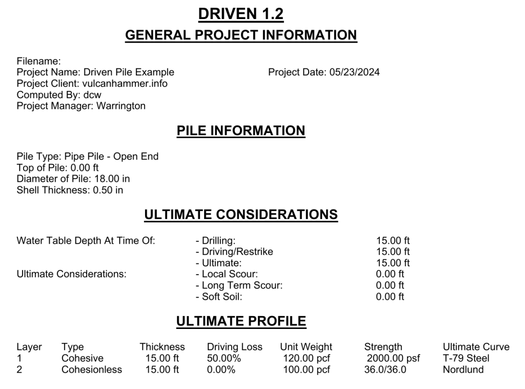
From here the soil profile is constructed.

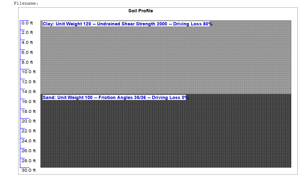
The upper layer is analysed using Tomlinson’s method and the lower Nordlund’s because of their respective soils. When they are applied to the pile the following bearing capacity graphs result.

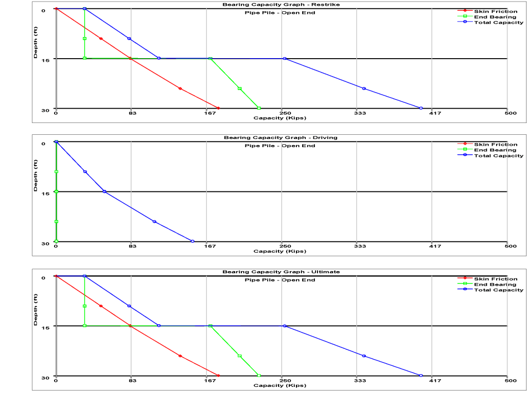
There are three of these:

Restrike, which is done after any set-up in the soils has dissipated. Set-up will be discussed when we get to pile dynamics an drivability.
Driving, which documents the soil resistance to driving (SRD) as opposed to the ultimate capacity. Pile driving induces various effects in the soil which again will be discussed when we get to drivability.
Ultimate, which is the main objective of this part of the study. If scour and other effects are not present, this will be identical to the restrike, as is the case here.

The graph documents the skin/shaft friction, end/toe bearing and total capacity/resistance as a function of depth. The deeper the pile penetrates, the higher the resistance. A detailed output can be found here. In this case the tip elevation (distance from the ground surface to the pile toe) is known. If it is necessary, for example, to design a pile to a certain ultimate capacity, then the graph can be developed at a deep tip elevation and then a tip elevation where the desired ultimate capacity can be found.

Such graphs are common with driven pile capacity analysis and drivability studies.

Summing Up the Results

The results can be summed up as follows:

Method	Cohesive Shaft Capacity Q_s1, kips	Cohesionless Shaft Capacity Q_s2, kips	Toe Capacity Q_p, kips	Total Capacity Q, kips
Dennis and Olson	48.4	52.8	13.3	114.5
Fellenius	14.6	67.7	40.6	122.9
FHWA/ Nordlund/ Tomlinson	82.3	97.8	224.7	404.8

Dennis and Olson’s and Fellenius’ Methods are fairly close, although they distribute the shaft resistance differently between the two layers. The outlier is the FHWA method. Part of the problem is that the properties given for the cohesive layer are unrealistic, as noted in the post Can Any Alpha Method be Converted to a Beta Method?

But such is to be expected of these methods; their multiplicity, like that of the dynamic formulae, are testaments to the fact that the science is anything but settled in this field.